信贷违约预测实战：从数据清洗到XGBoost调优全流程

文章目录

信贷违约预测实战：从数据清洗到XGBoost调优全流程一、项目背景二、数据探索与预处理1. 数据加载与基础检查2. 特征清理
三、数据与特征处理四、构建模型五、XGBoost调优实战1.基础参数设置2. 贝叶斯优化调参3. 最佳参数4. 最终模型评估
六、完整代码仓库

一、项目背景

精准预测用户贷款违约风险是风控系统的核心。本文将带您完整复现一个信贷违约预测项目，从数据清洗、特征工程到模型调优，最终实现高精度预测。项目使用Python，基于天池信贷数据集，全程手把手教学。

二、数据探索与预处理

1. 数据加载与基础检查


import pandas as pd
import numpy as np

读取数据，删除无关列


df = pd.read_csv('data/train.csv').drop(['id', 'issueDate'], axis=1)

检查数据基本信息


# 数据基本信息探索
df.info()
df.describe()
df.dtypes.value_counts()
# 找出有缺失值的特征
df.isnull().sum()
# 缺失值比例
df.isna().mean()

关键发现：

20列含缺失值（最高缺失率5.8%：employmentLength）4列非数值型（grade, subGrade, employmentLength,earliesCreditLine）policyCode列值无变化，需删除，n11,n12列类似，需删除

2. 特征清理

删除无用特征


df = df.drop(columns=['policyCode', 'n11', 'n12'])

处理earliesCreditLine列，提取年份


df['earliesCreditLine']=df['earliesCreditLine'].apply(lambda s: int(s[-4:]))

三、数据与特征处理

可以通过业务经验或者金融相关知识构建一些新特征或者交互项等，由于篇幅有限，这里不再赘述，希望大家发挥主观能动性！！！


# 自变量与因变量分离
y=df.pop('isDefault')

缺失值填充
类别型变量：用众数填充


cat_cols = ['grade', 'subGrade', 'employmentLength']
for col in cat_cols:
df[col].fillna(df[col].mode()[0], inplace=True)

数值型变量：用中位数填充


num_cols = df.select_dtypes(include=['float64', 'int64']).columns
for col in num_cols:
	if df[col].isnull().sum() > 0:
		df[col].fillna(df[col].median(), inplace=True)

类别型变量编码grade编码（A-G）


grade_map = {'A': 0, 'B': 1, 'C': 2, 'D': 3, 'E': 4, 'F': 5, 'G': 6}
df['grade'] = df['grade'].map(grade_map)

subGrade编码（按A1-A5, B1-B5…顺序）


subGrade_map = {}
for i, grade in enumerate(['A', 'B', 'C', 'D', 'E', 'F', 'G']):
	for j in range(1, 6):
		subGrade_map[f'{grade}{j}'] = i5 + j-1
		df['subGrade'] = df['subGrade'].map(subGrade_map)

employmentLength编码（<1年=0, 1年=1…10+年=10）


emp_length_map = {
'< 1 year': 0, '1 year': 1, '2 years': 2, '3 years': 3, '4 years': 4,
'5 years': 5, '6 years': 6, '7 years': 7, '8 years': 8, '9 years': 9,
'10+ years': 10
}
df['employmentLength'] = df['employmentLength'].map(emp_length_map)

编码逻辑：
grade：A(0) < B(1) < C(2) < … < G(6)
subGrade：A1(0), A2(1), …, A5(4), B1(5), B2(6)… G5(34)
employmentLength：按年限升序映射

四、构建模型


from sklearn.model_selection import train_test_split,StratifiedKFold
from sklearn.linear_model import LogisticRegression
from sklearn.tree import DecisionTreeClassifier
from sklearn.ensemble import RandomForestClassifier
from xgboost.sklearn import XGBClassifier
from lightgbm import LGBMClassifier
from sklearn.metrics import classification_report,roc_auc_score

判断因变量是否类别平衡


y.value_counts()/y.count()

为XGBoost设置权重
scale_pos_weight = y.value_counts()[0] / y.value_counts()[1]
模型对比


models = {
'log_model': LogisticRegression(max_iter=5000,random_state=42),
'tree':DecisionTreeClassifier(random_state=42),
'RF':RandomForestClassifier( random_state=42),
'XGB':XGBClassifier(random_state=42),
'lgb':LGBMClassifier(random_state=42)
}

以auc为评估指标来判断模型性能

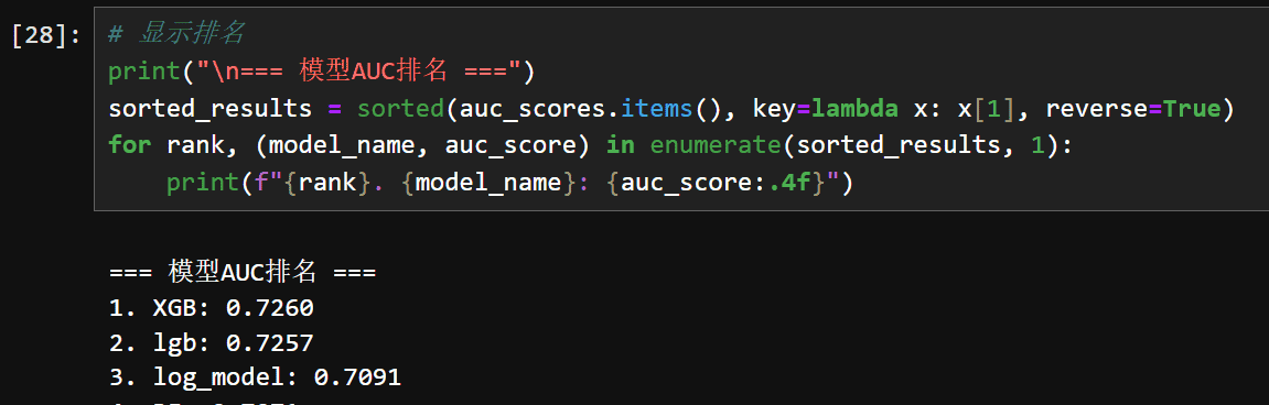
数据质量应该不太好，所以auc都不是很高，进一步构造特征等措施，auc提升的也不多。

结论：XGBoost表现最佳，选择其作为基础模型

五、XGBoost调优实战

1.基础参数设置


# XGBoost基础参数
xgb_base_params = {
     'objective': 'binary:logistic',
     'eval_metric': 'auc',
     'tree_method': 'hist', 
    'n_jobs': -1,
    'scale_pos_weight': scale_pos_weight,
     'random_state': 42,
     'verbosity': 0
}

2. 贝叶斯优化调参


from bayes_opt import BayesianOptimization

def xgb_cv(n_estimators, max_depth, learning_rate,min_child_weight, subsample, colsample_bytree, gamma, reg_alpha, reg_lambda):
	params = {**xgb_base_params,
	'n_estimators': int(n_estimators),
	'max_depth': int(max_depth),
	'learning_rate': learning_rate,
	'subsample': subsample,
	'colsample_bytree': colsample,
	'scale_pos_weight': scale_pos_weight,
	'objective': 'binary:logistic',
	'random_state': 42,
	'gamma': gamma,
	'reg_alpha': reg_alpha,
	'reg_lambda': reg_lambda
	}

	#3折交叉验证
	scores = []
	for train_idx, val_idx in StratifiedKFold(3).split(X_train, y_train):
		X_train_fold, X_val_fold = X_train.iloc[train_idx], X_train.iloc[val_idx]
		y_train_fold, y_val_fold = y_train.iloc[train_idx], y_train.iloc[val_idx]
	
	model = XGBClassifier(params)
	model.fit(X_train_fold, y_train_fold)
	scores.append(roc_auc_score(y_val_fold, model.predict_proba(X_val_fold)[:, 1]))
	
	return np.mean(scores)

定义搜索空间


pbounds = {
'n_estimators': (100, 500),
'max_depth': (3, 10),
'learning_rate': (0.01, 0.3),
'subsample': (0.6, 1.0),
'colsample': (0.6, 1.0)
}

执行优化


optimizer = BayesianOptimization(f=xgb_cv, pbounds=pbounds, random_state=42)
optimizer.maximize(init_points=10, n_iter=20)

3. 最佳参数


# 获取最佳参数
xgb_best_params = {**xgb_base_params}
xgb_best_params.update(xgb_optimizer.max['params'])
xgb_best_params['n_estimators'] = int(xgb_best_params['n_estimators'])
xgb_best_params['max_depth'] = int(xgb_best_params['max_depth'])

print("XGBoost最佳参数:")
for k, v in xgb_best_params.items():
     print(f"  {k}: {v}")

4. 最终模型评估

训练最终模型


final_model = XGBClassifier(
**xgb_best_params,early_stopping_rounds=50)
final_model.fit(X_train, y_train,
eval_set=[(X_val, y_val)],
verbose=False)
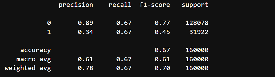
#测试集评估
print(classification_report(Ytest, final_model.predict(Xtest))) 
print("AUC: ", roc_auc_score(Ytest, final_model.predict_proba(Xtest)[:, 1]))

最终结果：