
1、实验原理
SIFT,即尺度不变特征变换,是用于图像处理领域的一种描述。这种描述具有尺度不变性,它对物体的尺度变化,刚体变换,光照强度和遮挡都具有较好的稳定性,可在图像中检测出关键点,是一种局部特征描述子。SIFT 算法被认为是图像匹配效果好的方法之 一算法实现特征匹配主要有三个流程:
①特征点提取; ②特征点主方向确定; ③特征点描述; ④特征点匹配;
其中特征点提取主要包括生成高斯差分(DOG)尺度空间、寻找局部极值点、特征点筛选、确定特征点方向;特征点匹配主要包括根据描述子相似性进行匹配、匹配对比值提纯、RANSAC方法剔除离群匹配对。
1.1 特征点提取
两种图像在匹配的时候可能因为拍摄的距离、拍摄的角度问题,会导致在特征点提取的时候差异很大,所以我们希望SIFT的特征点可以具有尺度不变性和方向不变性。 对于我们人类来说,在一定的范围内,无论物体远还是近,我们都可以一眼分辨出来,当一个人从远处走来的时候,我们可以从轮廓就判断出这是一个人,但是还看不清细节,当他走进的时候,我们才会去注意其他的细节特征。而计算机没有主观意识去识别哪里是特征点,它能做的,只是分辨出变化率最快的点。彩色图是三通道的,不好检测突变点。需要将RGB图转换为灰度图,此时灰度图为单通道,灰度值在0~255之间分布。而且当图像放大或者缩小时,它读取的特征点与原先可能差异很大,所以其中一个办法就是把物体的尺度空间图像集合提供给计算机,让它针对考虑不同尺度下都存在的特征点。
1.1.1 尺度空间
尺度空间的基本思想为:高斯核是唯一可以产生多尺度空间的核,在输入的图像模型中,通过高斯模糊函数连续的对尺度进行参数变换,最终得到多尺度空间序列。图像中某一尺度的空间函数 L(x ,y, σ)由可变参数的高斯函数 G(x, y, σ)和原输入图像I(x ,y)卷积得出:

其中,σ 表示为尺度空间因子,σ 越小,反应的局部点越清晰。反之 σ 越大,图像越模糊,越不能反应出图像的细节。
1.1.2 多分辨率图像金字塔
在早期图像的多尺度通常使用图像金字塔表述形式。图像金字塔是同一图象在不同的分辨率下得到的一组结果,其生成过程一半包含两个步骤: (1)对图像做高斯平滑(高斯模糊)。 (2)对图像做降采样,降维采样后得到一系列尺寸不断缩小的图像。

传统的SIFT算法是通过建立高斯差分函数(DOG) 方法来提取特征点。首先,在不同尺度参数的组数中,高斯差分图像是由某一相同尺度层的相邻图像作差值 得出。然后,将得到的差分图像与原图像 I(x, y)做卷积得到公式(3)的 DOG 函数:
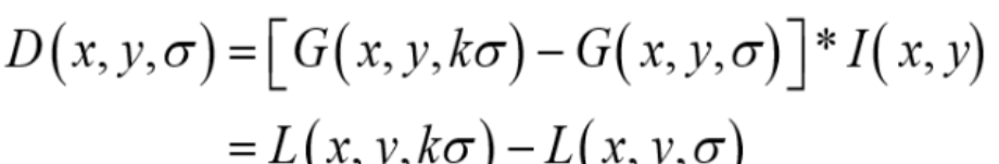
从上式可以知道,将相邻的两个高斯空间的图像相减就得到了DoG的响应图像。为了得到DoG图像,先要构造高斯尺度空间,而高斯的尺度空间可以在图像金字塔降维采样的基础上加上高斯滤波得到,也就是对图像金字塔的每层图像使用不同的尺度参数σ进行高斯模糊,使每层金字塔有多张高斯模糊过的图像,然后我们把得到的同一尺寸大小的图像划分为一组。
1.1.3 DOG局部极值检测
特征点是由DOG空间的局部极值点组成的。为了寻找DoG函数的极值点, 每一个像素点要和它所有的相邻点比较,看其是否比它的图像域和尺度域的相邻点大或者小。
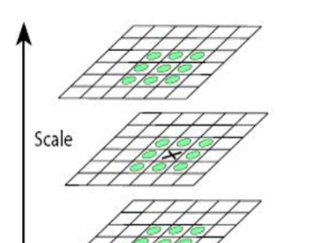
中间的检测点和它同尺度的8个相邻点和上下相邻尺度对应的9×2个 点共26个点比较,以确保在尺度空间和二维图像空间都检测到极值点。
特征点提取可以概括为以下几个步骤:
①构建高斯尺度空间,产生不同尺度的高斯模糊图像。
②进行降采用,得到一系列尺寸不断缩小的图像。
③DOG空间极值检测,去除部分边缘响应点。
1.2 特征点主方向的确定
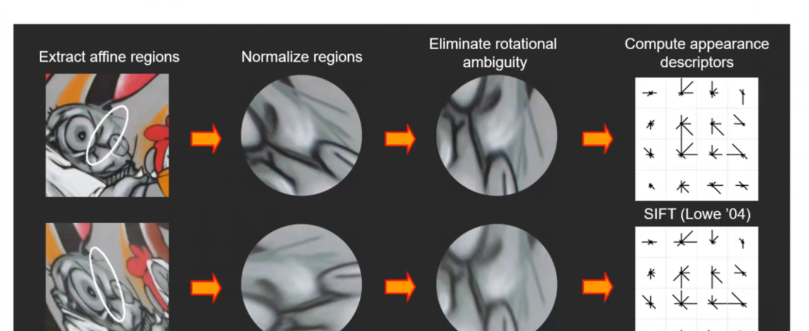
可以看到针对于房屋这个例子,要比较尺度里面的内容是比较容易的,因为它没有经过视角变换,只有尺度的变换,也就是只做了放大放小的操作,里面的内容基本一致。但是看到涂鸦的这个例子是进行了视角变换的,那么想要比较里面的内容,首先的一个思想就是将这个尺度变为同等大小的圆,在比较里面的内容。
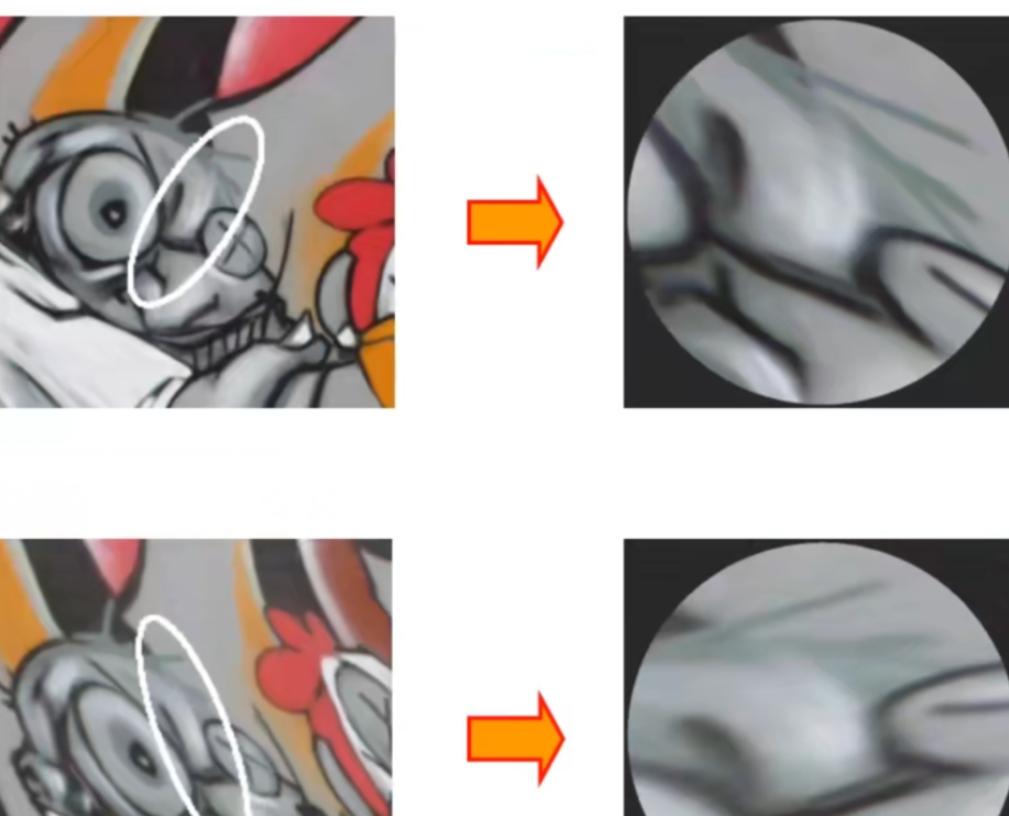
上图就是将两个尺度变为了同等大小的圆,可以看到里面的内容基本上是一致的,但是角度还是不同,这样仍然没有办法进行特征匹配。
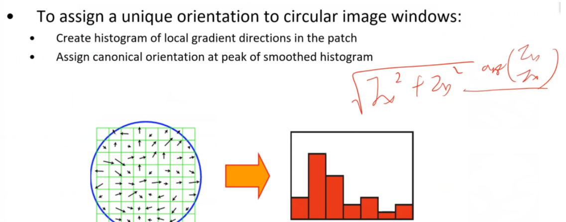
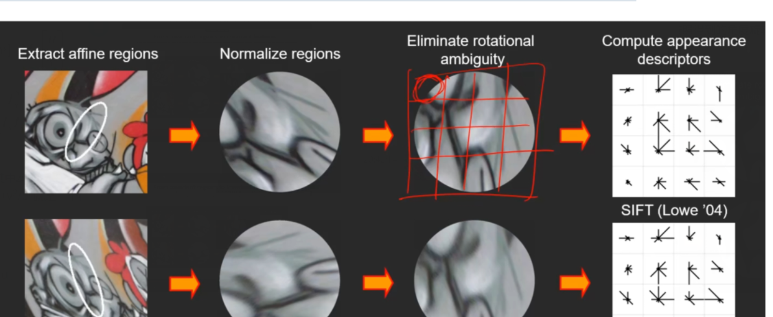
针对上述的角度问题,我们还需要对加了仿射变换的sift进一步进行扩展,使得其对于角度变换也具有协变性。具体怎样扩展可以看到上图,绿色的网格代表着图像上的每一个像素点,我们需要把每个像素点的梯度方向和梯度幅值都计算出来,然后绘制右边的梯度方向直方图。具体的绘制方法就是将横坐标制定为角度,范围为0-360°,将其按照45°一个格子进行量化,然后将每个像素点的梯度幅值投票到对应的梯度方向的直方图的格子里面去。将直方图绘制完之后,找到直方图里投票数最大对应的角度值,这也是图像梯度变换最大的方向,然后将图像的这个方向按照得到的角度旋转至0°的位置。
上图就是将尺度里面的每一个像素点梯度方向和梯度幅值都计算出来,然后绘制出梯度方向直方图,找到了梯度变换最大的方向对应的角度,再将图像的这个方向按照得到的角度旋转至0°的位置,就可以得到如上图的效果,可以看出尺度里的内容基本一致了,就可以进行匹配了。
1.3 特征点的描述
通过以上步骤,对于每一个关键点,拥有三个信息:位置、尺度以及方向。接下来就是为每个关键点建立一个描述符,使其不随各种变化而改变,比如光照变化、视角变化等等。并且描述符应该有较高的独特性,以便于提高特征点正确匹配的概率。
现在已将讲了使得sift对旋转变换、视角变换、尺度变换具有协变性的方法,下面谈一下光照的问题(之前讲的对于旋转、平移、光照具有不变性的是Harris角点检测,这并不意味着sift也具有相同的特性)。
针对于光照的问题,sift还做了进一步的扩展,也就是用sift描述符来描述尺度里面的内容。具体的做法就是将尺度区域化为一个nxn的格子图,如上图就是将尺度区域化为了4×4的格子图,那么对于每一个格子里面包含的每一个像素点我们也计算它的梯度方向和梯度幅值,然后画出针对于这个格子的梯度方向直方图(上面画的梯度方向直方图是针对于整个图像的),例如梯度方向直方图将角度分为了8组(0°-45°、45°-90°……315°-360°),每一组都有对应的投票值,我们就将每一组的投票值在每组方向上都绘制出来,如

进而画出整个尺度区域每个方格里面的类似于
的符号。画完之后我们就可以得到这样的一个4×4的方格
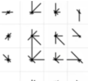
里面每一个格子都是8个方向的直方图,那么一共16个格子,就可以组成一个128维的描述符,这就是sift描述符。那么就将上面的第一张图的128维的描述符与第二张图的128维的描述符进行对比,其实是将128维里面的每8维的一个直方图进行比较,因为直方图代表着梯度,那么就比直接将像素值进行比较要好一点。那么对应光照变化来说,例如白天下的像素灰度值是255,晚上只有100,那么像素值在光照变化下是相差很大的,但是它对应的梯度变换的相差值是比较小的,因此就利用梯度值(sift描述符)的比较代替像素值的比较,就可以克服光照变换的影响从而进行特征匹配。
sift描述符的应用场景不限于sift多尺度检测,还可以用于Harris角点检测、拉普拉斯多尺度检测,都是为了对光照变换具有协变性。
那么为什么制作sift描述符要针对于尺度区域不同的局部的梯度方向直方图,而不能针对于整个尺度区域的梯度方向直方图?举一个例子:“我爱中国”和“爱我中国”两句话展示的是不同的意思,如果针对于整句话进行匹配,可以匹配得到(字都一样),但是这两句话表达的意思并不相同,但是如果针对于整句话的局部进行匹配,可以看到只有中国两字匹配的上,这就表明局部的比较会更加准确。另外将尺度区域化为4×4的方格是通过实验得出来较好的值,并且0-360°的角度值也不要划分得太细或者太粗。
2、实验代码
在上一节的三维重建课程中,我学习了Harris角点的检测,那么在这里我将对照新学习的SIFT特征点检测与上一节学习的Harris角点检测进行对照学习。
2.1 Harris特征匹配代码
from pylab import *#导入pylab库,这是Matplotlib库的一部分,用于绘图和数据可视化。
from PIL import Image#导入Python Imaging Library (PIL) 的 Image 模块,用于图像处理。

#导入 harris 模块,其中包含了Harris角点检测相关的函数。
from PCV.localdescriptors import harris
#导入 imresize 函数,用于图像的调整大小。
from PCV.tools.imtools import imresize#

#打开名为 "1.jpg"和"2.jpg"的图像,将其转换为灰度图像,然后将其转换为 NumPy 数组。
im1 = array(Image.open("../pic/11.jpg").convert("L"))
im2 = array(Image.open("../pic/12.jpg").convert("L"))

# 将含有图像信息的数组缩小以加快匹配速度
im1 = imresize(im1, (im1.shape[1]/2, im1.shape[0]/2))
im2 = imresize(im2, (im2.shape[1]/2, im2.shape[0]/2))

wid = 5#设置窗口大小为 5。
#计算图像 im1 中的 Harris 角点响应。
harrisim = harris.compute_harris_response(im1, 5)
#获取在 im1 中的 Harris 角点坐标。
fi#、ltered_coords1 = harris.get_harris_points(harrisim, wid+1)
#获取 im1 中 Harris 角点的描述子。
d1 = harris.get_descriptors(im1, filtered_coords1, wid)

#类似地,对 im2 进行 Harris 角点检测,获得在 im2 中的角点坐标和描述子。
harrisim = harris.compute_harris_response(im2, 5)
filtered_coords2 = harris.get_harris_points(harrisim, wid+1)
d2 = harris.get_descriptors(im2, filtered_coords2, wid)

print ('starting matching')
#使用双向匹配算法匹配两幅图像中的特征点。
matches = harris.match_twosided(d1, d2)

#绘制匹配结果
figure()
suptitle("Harris matching")
gray()
harris.plot_matches(im1, im2, filtered_coords1, filtered_coords2, matches)
show()
2.2 SIFT特征匹配代码:
2.2.1 方法一(直接调用PCV库里面sift算法)
①安装PCV:
下载PCV包链接:https://codeload.github.com/Li-Shu14/PCV/zip/master;
不用解压,copy到项目文件夹下;
项目文件夹下运行cmd,conda activate进入指定虚拟环境,执行以下命令安装:
pip install PCV-master.zip
②安装vlfeat:
下载地址:VLFeat – Home;
下载0.9.20版本,即vlfeat-0.9.20-bin.tar.gz
③解压后进入bin文件夹,根据系统选择对应版本,很重要!!!将对应版本文件夹复制到项目文件夹下,这边将其重新命名为win64vlfeat;
④找到PCV包下localdescriptors文件夹下的sift.py文件,找到下面这段代码:
def process_image(imagename,resultname,params="--edge-thresh 10 --peak-thresh 5"):
    """ Process an image and save the results in a file. """

    if imagename[-3:] != 'pgm':
        # create a pgm file
        im = Image.open(imagename).convert('L')
        im.save('tmp.pgm')
        imagename = 'tmp.pgm'

    cmmd = str(r"D:python projectSIFTwin64vlfeatsift.exe "+imagename+" --output="+resultname+
                " "+params)
    os.system(cmmd)
    print('processed', imagename, 'to', resultname)
将其中cmmd后的sift.exe文件路径改为上一步路径,注意路径前加r,sift.exe后有空格
⑤下述代码就是调用PCV包里面的sift函数来实现的sift特征匹配
from PIL import Image
# from numpy import *
from pylab import *
import os
import numpy as np


def process_image(imagename, resultname, params="--edge-thresh 10 --peak-thresh 5"):
    """ Process an image and save the results in a file. """

    if imagename[-3:] != 'pgm':
        # create a pgm file
        im = Image.open(imagename).convert('L')  # .convert('L') 将RGB图像转为灰度模式,灰度值范围[0,255]
        im.save('tmp.pgm')  # 将灰度值图像信息保存在.pgm文件中
        imagename = 'tmp.pgm'

    cmmd = str(r"H:/2023.4sift/win64vlfeat/sift.exe " + imagename + " --output=" + resultname +
               " " + params)
    os.system(cmmd)  # 执行sift可执行程序,生成resultname(test.sift)文件
    print('processed', imagename, 'to', resultname)


def read_features_from_file(filename):
    """ Read feature properties and return in matrix form. """
    # print(filename)
    f = np.loadtxt(filename)
    return f[:, :4], f[:, 4:]  # feature locations, descriptors


def plot_features(im, locs, circle=True):
    """ Show image with features. input: im (image as array),
        locs (row, col, scale, orientation of each feature). """

    def draw_circle(c, r):
        t = arange(0, 1.01, .01) * 2 * pi
        x = r * cos(t) + c[0]
        y = r * sin(t) + c[1]
        plot(x, y, 'b', linewidth=2)

    imshow(im)
    if circle:
        for p in locs:
            draw_circle(p[:2], p[2])
    else:
        plot(locs[:, 0], locs[:, 1], 'ob')
    axis('off')


def match(desc1, desc2):
    """对于第一幅图像中的每个描述子,选取其在第二幅图像中的匹配
    输入:desc1(第一幅图像中的描述子),desc2(第二幅图像中的描述子)"""
    desc1 = array([d / linalg.norm(d) for d in desc1])
    desc2 = array([d / linalg.norm(d) for d in desc2])

    dist_ratio = 0.6
    desc1_size = desc1.shape
    matchscores = zeros((desc1_size[0], 1), 'int')
    desc2t = desc2.T  # 预先计算矩阵转置
    for i in range(desc1_size[0]):
        dotprods = dot(desc1[i, :], desc2t)  # 向量点乘
        dotprods = 0.9999 * dotprods
        # 反余弦和反排序,返回第二幅图像中特征的索引
        indx = argsort(arccos(dotprods))

        # 检查最近邻的角度是否小于dist_ratio乘以第二近邻的角度
        if arccos(dotprods)[indx[0]] < dist_ratio * arccos(dotprods)[indx[1]]:
            matchscores[i] = int(indx[0])

    return matchscores


def match_twosided(desc1, desc2):
    """双向对称版本的match()"""
    matches_12 = match(desc1, desc2)
    matches_21 = match(desc2, desc1)

    ndx_12 = matches_12.nonzero()[0]

    # 去除不对称的匹配
    for n in ndx_12:
        if matches_21[int(matches_12[n])] != n:
            matches_12[n] = 0

    return matches_12


def appendimages(im1, im2):
    """返回将两幅图像并排拼接成的一幅新图像"""
    # 选取具有最少行数的图像,然后填充足够的空行
    rows1 = im1.shape[0]
    rows2 = im2.shape[0]

    if rows1 < rows2:
        im1 = concatenate((im1, zeros((rows2 - rows1, im1.shape[1]))), axis=0)
    elif rows1 > rows2:
        im2 = concatenate((im2, zeros((rows1 - rows2, im2.shape[1]))), axis=0)
    return concatenate((im1, im2), axis=1)


def plot_matches(im1, im2, locs1, locs2, matchscores, show_below=True):
    """ 显示一幅带有连接匹配之间连线的图片
        输入:im1, im2(数组图像), locs1,locs2(特征位置),matchscores(match()的输出),
        show_below(如果图像应该显示在匹配的下方)
    """
    im3 = appendimages(im1, im2)
    if show_below:
        im3 = vstack((im3, im3))

    plt.figure(figsize=(20, 10))
    imshow(im3)

    cols1 = im1.shape[1]
    for i in range(len(matchscores)):
        if matchscores[i] > 0:
            plot([locs1[i, 0], locs2[matchscores[i, 0], 0] + cols1], [locs1[i, 1], locs2[matchscores[i, 0], 1]], 'c')
    axis('off')


if __name__ == '__main__':
    # imname = (r'H:2023.4sift2.jpg')  # 待处理图像路径
    # im = Image.open(imname)
    # process_image(imname, 'out_sift_2.txt')
    # l1, d1 = read_features_from_file('out_sift_2.txt')
    # figure()
    # gray()
    # plot_features(im, l1, circle=True)
    # title('sift-features')
    # show()
    im1f = r'H:2023.4sift1.jpg'
    im2f = r'H:2023.4sift2.jpg'
    im1 = array(Image.open(im1f))
    im2 = array(Image.open(im2f))

    # process_image(im1f, 'out_sift_1.txt')
    l1, d1 = read_features_from_file('out_sift_1.txt')
    figure()
    gray()
    plt.figure(figsize=(20, 10))
    subplot(121)
    plot_features(im1, l1, circle=False)

    # process_image(im2f, 'out_sift_2.txt')
    l2, d2 = read_features_from_file('out_sift_2.txt')
    subplot(122)
    plot_features(im2, l2, circle=False)
    matches = match_twosided(d1, d2)
    print('{} matches'.format(len(matches.nonzero()[0])))
    figure()
    gray()
    plot_matches(im1, im2, l1, l2, matches, show_below=True)

    show()
⑥执行上述代码,失败了,总是找不到文件out_sift_1.txt。这个文件是调用PCV包里的 SIFT 算法处理第一个图像,并将特征保存到名为 'out_sift_1.txt' 的文件中,没有这个文件,说明sift算法没调用起,调了一天还是没有调出来就放弃了。
FileNotFoundError: out_sift_1.txt not found.
2.2.2 方法二:根据sift算法的原理编写的代码,而没有调用PCV包里现有的sift算法
方法二的代码如下:
import warnings

warnings.filterwarnings("ignore")  # 忽略警告
import numpy as np
import matplotlib.pyplot as plt
from PIL import Image

#下列函数通过对输入图像进行卷积操作,返回卷积结果。
def convolve(kernel, img, padding, strides):
    result = None
    kernel_size = kernel.shape
    img_size = img.shape
#如果输入图像是三通道的,函数会对每个通道进行独立的卷积操作,然后将结果合并为一个三通道的输出。
    if len(img_size) == 3:
        channel = []
#在卷积操作中,函数使用了填充(padding)和步长(strides)来调整卷积的输出大小。
        for i in range(img_size[-1]):
            pad_img = np.pad(img[:, :, i], ((padding[0], padding[1]), (padding[2], padding[3])), 'constant')
            temp = []
            for j in range(0, img_size[0], strides[1]):
                temp.append([])
                for k in range(0, img_size[1], strides[0]):
                    val = (kernel * pad_img[j * strides[1]:j * strides[1] + kernel_size[0],
                                    k * strides[0]:k * strides[0] + kernel_size[1]]).sum()
                    temp[-1].append(val)
            channel.append(np.array(temp))

        channel = tuple(channel)
        result = np.dstack(channel)
#如果输入图像是二维的,函数会对其进行单通道卷积操作。
    elif len(img_size) == 2:
        channel = []
#在卷积操作中,函数使用了填充(padding)和步长(strides)来调整卷积的输出大小。
        pad_img = np.pad(img, ((padding[0], padding[1]), (padding[2], padding[3])),
                         'constant')
        for j in range(0, img_size[0], strides[1]):
            channel.append([])
            for k in range(0, img_size[1], strides[0]):
                val = (kernel * pad_img[j * strides[1]:j * strides[1] + kernel_size[0],
                                k * strides[0]:k * strides[0] + kernel_size[1]]).sum()
                channel[-1].append(val)
        result = np.array(channel)
    return result


# 降采样,隔点取点(通过降采样可以提升sift检测的速度,因为可以只制定几个DOG模板,DOG模板没有变得很大(第一个加速原因),还把图像像素点减少了(第二个加速原因),这两点都使得卷积的速度更快)
def undersampling(img, step=2):
    return img[::step, ::step]


# DOG模板是用两个高斯核相减得到的,所以首先要产生高斯核
def GuassianKernel(sigma, dim):
    '''
    :param sigma: 标准差
    :param dim: 高斯核的纬度(必须是个奇数)
    :return: 返回高斯核
    '''
    temp = [t - (dim // 2) for t in range(dim)]  # 生成二维高斯的x与y
    assistant = []
    for i in range(dim):
        assistant.append(temp)
    assistant = np.array(assistant)
    temp = 2 * sigma * sigma
    result = (1.0 / (temp * np.pi)) * np.exp(-(assistant ** 2 + (assistant.T) ** 2) / temp)  # 二维高斯公式
    return result

# 通过上面定义的产生高斯核的函数,得到高斯金字塔和高斯差分金字塔(DOG)
def getDoG(img, n, sigma0, S=None, O=None):
    if S == None:
        S = n + 3  # 至少有4张 (第一张和最后一张高斯金字塔无法提取特征,差分以后的第一张和最后一张也无法提取特征)
    if O == None:
        O = int(np.log2(min(img.shape[0], img.shape[1]))) - 3  # 计算最大可以计算多少层 O=log2(min(img长,img宽))-3

    k = 2 ** (1.0 / n)
    sigma = [[(k ** s) * sigma0 * (1 << o) for s in range(S)] for o in range(O)]  # 每一层 sigma按照 k^1/s * sigama0  排列 下一层的sigma都要比上一层sigma大两倍
    sample = [undersampling(img, 1 << o) for o in range(O)]  # 降采样取图片作为该层的输入

    Guass_Pyramid = []
    for i in range(O):
        Guass_Pyramid.append([])  # 申明二维空数组
        for j in range(S):
            dim = int(6*sigma[i][j] + 1) # 上网查找相关信息 高斯核大小随sigma变化的效果更好
            #dim = int(9)
            if dim % 2 == 0:  # 防止输入的高斯核不是奇数
                dim += 1
            Guass_Pyramid[-1].append(convolve(GuassianKernel(sigma[i][j], dim), sample[i], [dim // 2, dim // 2, dim // 2, dim // 2], [1, 1]))  # 在第i层添加第j张 经过高斯卷积的 该图片四周扩展 5//2=2 用于高斯卷积
    DoG_Pyramid = [[Guass_Pyramid[o][s + 1] - Guass_Pyramid[o][s] for s in range(S - 1)] for o in range(O)]  #每一层中 上一张减去下一张得到差分高斯核

    return DoG_Pyramid, Guass_Pyramid, O  # 返回高斯金字塔和高斯差分金字塔

# 下列函数是SIFT算法中的局部极值点的调整过程
#DoG:高斯差分金字塔。o:金字塔的组号。s:组内的层数。x、y:候选极值点的坐标。contrastThreshold:对比度阈值,用于剔除低对比度的极值点。edgeThreshold:边缘阈值,用于剔除边缘上的极值点。sigma:高斯模糊的标准差。n:每组的层数。SIFT_FIXPT_SCALE:SIFT固定点尺度。
def adjustLocalExtrema(DoG, o, s, x, y, contrastThreshold, edgeThreshold, sigma, n, SIFT_FIXPT_SCALE):
    SIFT_MAX_INTERP_STEPS = 5
    SIFT_IMG_BORDER = 5

    point = []

    img_scale = 1.0 / (255 * SIFT_FIXPT_SCALE)
    deriv_scale = img_scale * 0.5
    second_deriv_scale = img_scale
    cross_deriv_scale = img_scale * 0.25

    img = DoG[o][s]
    i = 0
    while i < SIFT_MAX_INTERP_STEPS:
        if s < 1 or s > n or y < SIFT_IMG_BORDER or y >= img.shape[1] - SIFT_IMG_BORDER or x < SIFT_IMG_BORDER or x >=
                img.shape[0] - SIFT_IMG_BORDER:
            return None, None, None, None

        img = DoG[o][s]
        prev = DoG[o][s - 1]
        next = DoG[o][s + 1]

        dD = [(img[x, y + 1] - img[x, y - 1]) * deriv_scale,
              (img[x + 1, y] - img[x - 1, y]) * deriv_scale,
              (next[x, y] - prev[x, y]) * deriv_scale]

        v2 = img[x, y] * 2
        dxx = (img[x, y + 1] + img[x, y - 1] - v2) * second_deriv_scale
        dyy = (img[x + 1, y] + img[x - 1, y] - v2) * second_deriv_scale
        dss = (next[x, y] + prev[x, y] - v2) * second_deriv_scale
        dxy = (img[x + 1, y + 1] - img[x + 1, y - 1] - img[x - 1, y + 1] + img[x - 1, y - 1]) * cross_deriv_scale
        dxs = (next[x, y + 1] - next[x, y - 1] - prev[x, y + 1] + prev[x, y - 1]) * cross_deriv_scale
        dys = (next[x + 1, y] - next[x - 1, y] - prev[x + 1, y] + prev[x - 1, y]) * cross_deriv_scale

        H = [[dxx, dxy, dxs],
             [dxy, dyy, dys],
             [dxs, dys, dss]]

        X = np.matmul(np.linalg.pinv(np.array(H)), np.array(dD))

        xi = -X[2]
        xr = -X[1]
        xc = -X[0]

        if np.abs(xi) < 0.5 and np.abs(xr) < 0.5 and np.abs(xc) < 0.5:
            break

        y += int(np.round(xc))
        x += int(np.round(xr))
        s += int(np.round(xi))

        i += 1

    if i >= SIFT_MAX_INTERP_STEPS:
        return None, x, y, s
    if s < 1 or s > n or y < SIFT_IMG_BORDER or y >= img.shape[1] - SIFT_IMG_BORDER or x < SIFT_IMG_BORDER or x >=
            img.shape[0] - SIFT_IMG_BORDER:
        return None, None, None, None

    t = (np.array(dD)).dot(np.array([xc, xr, xi]))

    contr = img[x, y] * img_scale + t * 0.5
    # 确定极值点位置第四步:舍去低对比度的点
    if np.abs(contr) * n < contrastThreshold:
        return None, x, y, s

    # 确定极值点位置第五步:边缘效应的去除。 利用Hessian矩阵的迹和行列式计算主曲率的比值
    tr = dxx + dyy
    det = dxx * dyy - dxy * dxy
    if det <= 0 or tr * tr * edgeThreshold >= (edgeThreshold + 1) * (edgeThreshold + 1) * det:
        return None, x, y, s

    point.append((x + xr) * (1 << o))
    point.append((y + xc) * (1 << o))
    point.append(o + (s << 8) + (int(np.round((xi + 0.5)) * 255) << 16))
    point.append(sigma * np.power(2.0, (s + xi) / n) * (1 << o) * 2)
#该函数的输出包括:point:找到的关键点的信息,包括位置、尺度等。x、y、s:调整后的极值点坐标和尺度。
    return point, x, y, s

#这个函数用于为关键点计算主方向,以确保后续描述子的旋转不变性。最终,主方向是通过计算梯度直方图的峰值确定的,峰值对应的方向即为关键点的主方向。
def GetMainDirection(img, r, c, radius, sigma, BinNum):
    expf_scale = -1.0 / (2.0 * sigma * sigma)

    X = []
    Y = []
    W = []
    temphist = []

    for i in range(BinNum):
        temphist.append(0.0)

    # 图像梯度直方图统计的像素范围
    k = 0
    for i in range(-radius, radius + 1):
        y = r + i
        if y <= 0 or y >= img.shape[0] - 1:
            continue
        for j in range(-radius, radius + 1):
            x = c + j
            if x <= 0 or x >= img.shape[1] - 1:
                continue

            dx = (img[y, x + 1] - img[y, x - 1])
            dy = (img[y - 1, x] - img[y + 1, x])

            X.append(dx)
            Y.append(dy)
            W.append((i * i + j * j) * expf_scale)
            k += 1

    length = k

    W = np.exp(np.array(W))
    Y = np.array(Y)
    X = np.array(X)
    Ori = np.arctan2(Y, X) * 180 / np.pi
    Mag = (X ** 2 + Y ** 2) ** 0.5

    # 计算直方图的每个bin
    for k in range(length):
        bin = int(np.round((BinNum / 360.0) * Ori[k]))
        if bin >= BinNum:
            bin -= BinNum
        if bin < 0:
            bin += BinNum
        temphist[bin] += W[k] * Mag[k]

    # smooth the histogram
    # 高斯平滑
    temp = [temphist[BinNum - 1], temphist[BinNum - 2], temphist[0], temphist[1]]
    temphist.insert(0, temp[0])
    temphist.insert(0, temp[1])
    temphist.insert(len(temphist), temp[2])
    temphist.insert(len(temphist), temp[3])  # padding

    hist = []
    for i in range(BinNum):
        hist.append(
            (temphist[i] + temphist[i + 4]) * (1.0 / 16.0) + (temphist[i + 1] + temphist[i + 3]) * (4.0 / 16.0) +
            temphist[i + 2] * (6.0 / 16.0))

    # 得到主方向
    maxval = max(hist)

    return maxval, hist

# 功能:这个函数实现了在图像中找到稳定的关键点
def LocateKeyPoint(DoG, sigma, GuassianPyramid, n, BinNum=36, contrastThreshold=0.04, edgeThreshold=10.0):
    SIFT_ORI_SIG_FCTR = 1.52
    SIFT_ORI_RADIUS = 3 * SIFT_ORI_SIG_FCTR
    SIFT_ORI_PEAK_RATIO = 0.8

    SIFT_INT_DESCR_FCTR = 512.0
    # SIFT_FIXPT_SCALE = 48
    SIFT_FIXPT_SCALE = 1

    KeyPoints = []
    O = len(DoG)
    S = len(DoG[0])
    for o in range(O):
        for s in range(1, S - 1):
            # 第一步:设定阈值
            threshold = 0.5 * contrastThreshold / (n * 255 * SIFT_FIXPT_SCALE)# 用于阈值化,去噪
            img_prev = DoG[o][s - 1]
            img = DoG[o][s]
            img_next = DoG[o][s + 1]
            for i in range(img.shape[0]):
                for j in range(img.shape[1]):
                    val = img[i, j]
                    eight_neiborhood_prev = img_prev[max(0, i - 1):min(i + 2, img_prev.shape[0]), max(0, j - 1):min(j + 2, img_prev.shape[1])]
                    eight_neiborhood = img[max(0, i - 1):min(i + 2, img.shape[0]), max(0, j - 1):min(j + 2, img.shape[1])]
                    eight_neiborhood_next = img_next[max(0, i - 1):min(i + 2, img_next.shape[0]), max(0, j - 1):min(j + 2, img_next.shape[1])]
                    # 第二步:阈值化,在高斯差分金字塔中找极值
                    if np.abs(val) > threshold and
                            ((val > 0 and (val >= eight_neiborhood_prev).all() and (val >= eight_neiborhood).all() and (
                                    val >= eight_neiborhood_next).all())
                             or (val < 0 and (val <= eight_neiborhood_prev).all() and (
                                            val <= eight_neiborhood).all() and (val <= eight_neiborhood_next).all())): # 如果某点大于阈值,并且 比周围8个点、上下2*9个点共26个点都大或都小,则认为是关键点
                        # 第三步:精调位置,通过函数adjustLocalExtrema:实现
                        point, x, y, layer = adjustLocalExtrema(DoG, o, s, i, j, contrastThreshold, edgeThreshold,
                                                                sigma, n, SIFT_FIXPT_SCALE)
                        if point == None:
                            continue
                        scl_octv = point[-1] * 0.5 / (1 << o)
                        # GetMainDirection:(确定极值点的位置以后就)求主方向
                        omax, hist = GetMainDirection(GuassianPyramid[o][layer], x, y,
                                                      int(np.round(SIFT_ORI_RADIUS * scl_octv)),
                                                      SIFT_ORI_SIG_FCTR * scl_octv, BinNum)
                        mag_thr = omax * SIFT_ORI_PEAK_RATIO
                        for k in range(BinNum):
                            if k > 0:
                                l = k - 1
                            else:
                                l = BinNum - 1
                            if k < BinNum - 1:
                                r2 = k + 1
                            else:
                                r2 = 0
                            if hist[k] > hist[l] and hist[k] > hist[r2] and hist[k] >= mag_thr:
                                bin = k + 0.5 * (hist[l] - hist[r2]) / (hist[l] - 2 * hist[k] + hist[r2])
                                if bin < 0:
                                    bin = BinNum + bin
                                else:
                                    if bin >= BinNum:
                                        bin = bin - BinNum
                                temp = point[:]
                                temp.append((360.0 / BinNum) * bin)
                                KeyPoints.append(temp)

    return KeyPoints


#实现了SIFT算法中计算关键点描述子的函数,描述子包含了关键点周围区域的梯度信息,用于后续的特征匹配。
def calcSIFTDescriptor(img, ptf, ori, scl, d, n, SIFT_DESCR_SCL_FCTR=3.0, SIFT_DESCR_MAG_THR=0.2,
                       SIFT_INT_DESCR_FCTR=512.0, FLT_EPSILON=1.19209290E-07):
    dst = []
    pt = [int(np.round(ptf[0])), int(np.round(ptf[1]))]  # 坐标点取整
    # 旋转到主方向
    cos_t = np.cos(ori * (np.pi / 180))  # 余弦值
    sin_t = np.sin(ori * (np.pi / 180))  # 正弦值
    bins_per_rad = n / 360.0
    exp_scale = -1.0 / (d * d * 0.5)
    hist_width = SIFT_DESCR_SCL_FCTR * scl
    # radius: 统计区域边长的一半
    radius = int(np.round(hist_width * 1.4142135623730951 * (d + 1) * 0.5))
    cos_t /= hist_width
    sin_t /= hist_width

    rows = img.shape[0]
    cols = img.shape[1]

    hist = [0.0] * ((d + 2) * (d + 2) * (n + 2))
    X = []
    Y = []
    RBin = []
    CBin = []
    W = []

    k = 0
    for i in range(-radius, radius + 1):
        for j in range(-radius, radius + 1):

            c_rot = j * cos_t - i * sin_t
            r_rot = j * sin_t + i * cos_t
            rbin = r_rot + d // 2 - 0.5
            cbin = c_rot + d // 2 - 0.5
            r = pt[1] + i
            c = pt[0] + j

            if rbin > -1 and rbin < d and cbin > -1 and cbin < d and r > 0 and r < rows - 1 and c > 0 and c < cols - 1:
                dx = (img[r, c + 1] - img[r, c - 1])
                dy = (img[r - 1, c] - img[r + 1, c])
                X.append(dx)
                Y.append(dy)
                RBin.append(rbin)
                CBin.append(cbin)
                W.append((c_rot * c_rot + r_rot * r_rot) * exp_scale)
                k += 1

    length = k
    Y = np.array(Y)
    X = np.array(X)
    Ori = np.arctan2(Y, X) * 180 / np.pi
    Mag = (X ** 2 + Y ** 2) ** 0.5
    W = np.exp(np.array(W))

    for k in range(length):
        rbin = RBin[k]
        cbin = CBin[k]
        obin = (Ori[k] - ori) * bins_per_rad
        mag = Mag[k] * W[k]

        r0 = int(rbin)
        c0 = int(cbin)
        o0 = int(obin)
        rbin -= r0
        cbin -= c0
        obin -= o0

        if o0 < 0:
            o0 += n
        if o0 >= n:
            o0 -= n

        # histogram update using tri-linear interpolation
        v_r1 = mag * rbin
        v_r0 = mag - v_r1

        v_rc11 = v_r1 * cbin
        v_rc10 = v_r1 - v_rc11

        v_rc01 = v_r0 * cbin
        v_rc00 = v_r0 - v_rc01

        v_rco111 = v_rc11 * obin
        v_rco110 = v_rc11 - v_rco111

        v_rco101 = v_rc10 * obin
        v_rco100 = v_rc10 - v_rco101

        v_rco011 = v_rc01 * obin
        v_rco010 = v_rc01 - v_rco011

        v_rco001 = v_rc00 * obin
        v_rco000 = v_rc00 - v_rco001

        idx = ((r0 + 1) * (d + 2) + c0 + 1) * (n + 2) + o0
        hist[idx] += v_rco000
        hist[idx + 1] += v_rco001
        hist[idx + (n + 2)] += v_rco010
        hist[idx + (n + 3)] += v_rco011
        hist[idx + (d + 2) * (n + 2)] += v_rco100
        hist[idx + (d + 2) * (n + 2) + 1] += v_rco101
        hist[idx + (d + 3) * (n + 2)] += v_rco110
        hist[idx + (d + 3) * (n + 2) + 1] += v_rco111

    # finalize histogram, since the orientation histograms are circular
    for i in range(d):
        for j in range(d):
            idx = ((i + 1) * (d + 2) + (j + 1)) * (n + 2)
            hist[idx] += hist[idx + n]
            hist[idx + 1] += hist[idx + n + 1]
            for k in range(n):
                dst.append(hist[idx + k])

    # copy histogram to the descriptor,
    # apply hysteresis thresholding
    # and scale the result, so that it can be easily converted
    # to byte array
    nrm2 = 0
    length = d * d * n
    for k in range(length):
        nrm2 += dst[k] * dst[k]
    thr = np.sqrt(nrm2) * SIFT_DESCR_MAG_THR

    nrm2 = 0
    for i in range(length):
        val = min(dst[i], thr)
        dst[i] = val
        nrm2 += val * val
    nrm2 = SIFT_INT_DESCR_FCTR / max(np.sqrt(nrm2), FLT_EPSILON) # 归一化
    for k in range(length):
        dst[k] = min(max(dst[k] * nrm2, 0), 255)

    return dst


# 计算sift描述符
def calcDescriptors(gpyr, keypoints, SIFT_DESCR_WIDTH=4, SIFT_DESCR_HIST_BINS=8):
    # SIFT_DESCR_WIDTH = 4,描述直方图的宽度
    # SIFT_DESCR_HIST_BINS = 8
    d = SIFT_DESCR_WIDTH
    n = SIFT_DESCR_HIST_BINS
    descriptors = []

    # keypoints(x,y,低8位组数次8位层数,尺度,主方向)
    for i in range(len(keypoints)):
        kpt = keypoints[i]
        o = kpt[2] & 255  # 组序号
        s = (kpt[2] >> 8) & 255  # 该特征点所在的层序号
        scale = 1.0 / (1 << o)  # 缩放倍数
        size = kpt[3] * scale  # 该特征点所在组的图像尺寸
        ptf = [kpt[1] * scale, kpt[0] * scale]  # 该特征点在金字塔组中的坐标
        img = gpyr[o][s]  # 该点所在的金字塔图像

        descriptors.append(calcSIFTDescriptor(img, ptf, kpt[-1], size * 0.5, d, n))  # calcSIFTDescriptor:更小的计算描述符函数
    return descriptors

#这个函数实现了完整的SIFT算法,包括建立高斯差分金字塔、确定关键点位置、为关键点赋予方向、计算关键点描述子等步骤。最终返回了图像中检测到的关键点及其对应的描述子。这些关键点和描述子可用于图像的特征匹配、物体识别等应用。
def SIFT(img, showDoGimgs=False):
    # 1. 建立高斯差分金字塔,
    SIFT_SIGMA = 1.6
    SIFT_INIT_SIGMA = 0.5  # 假设的摄像头的尺度
    sigma0 = np.sqrt(SIFT_SIGMA ** 2 - SIFT_INIT_SIGMA ** 2) #初始sigma0
    n = 2######

    DoG, GuassianPyramid,octaves = getDoG(img, n, sigma0)  # 函数1.1,getDoG:得到高斯金字塔和高斯差分金字塔

    if showDoGimgs:
        plt.figure(1)
        for i in range(octaves):
            for j in range(n + 3):
                array = np.array(GuassianPyramid[i][j], dtype=np.float32)
                plt.subplot(octaves, n + 3, j + (i) * octaves + 1)
                plt.imshow(array.astype(np.uint8), cmap='gray')
                plt.axis('off')
        plt.show()

        plt.figure(2)
        for i in range(octaves):
            for j in range(n + 2):
                array = np.array(DoG[i][j], dtype=np.float32)
                plt.subplot(octaves, n + 3, j + (i) * octaves + 1)
                plt.imshow(array.astype(np.uint8), cmap='gray')
                plt.axis('off')
        plt.show()

    #2. 确定关键点位置,为关键点赋予方向
    KeyPoints = LocateKeyPoint(DoG, SIFT_SIGMA, GuassianPyramid, n)  # 函数2.1,LocateKeyPoint:关键点定位

    #3. 计算关键点的描述符
    discriptors = calcDescriptors(GuassianPyramid, KeyPoints)  # 函数3.1,calcDescriptors:计算描述符

    return KeyPoints, discriptors

#该函数实现了在图像检测直线功能(检测匹配点之间的直线)。
def Lines(img, info, color=(255, 0, 0), err=700):
    if len(img.shape) == 2:
        result = np.dstack((img, img, img))
    else:
        result = img
    k = 0
    for i in range(result.shape[0]):
        for j in range(result.shape[1]):
            temp = (info[:, 1] - info[:, 0])
            A = (j - info[:, 0]) * (info[:, 3] - info[:, 2])
            B = (i - info[:, 2]) * (info[:, 1] - info[:, 0])
            temp[temp == 0] = 1e-9
            t = (j - info[:, 0]) / temp
            e = np.abs(A - B)
            temp = e < err
            if (temp * (t >= 0) * (t <= 1)).any():
                result[i, j] = color
                k += 1
    #print(k)

    return result

#该函数实现了在图像上绘制出检测到的直线的功能(将匹配点用直线连接起来)。
def drawLines(X1, X2, Y1, Y2, dis, img, num=10):
    info = list(np.dstack((X1, X2, Y1, Y2, dis))[0])
    info = sorted(info, key=lambda x: x[-1])
    info = np.array(info)
    info = info[:min(num, info.shape[0]), :]
    img = Lines(img, info)
    # plt.imsave('./sift/3.jpg', img)

    if len(img.shape) == 2:
        plt.imshow(img.astype(np.uint8), cmap='gray')
    else:
        plt.imshow(img.astype(np.uint8))
    plt.axis('off')
    # plt.plot([info[:,0], info[:,1]], [info[:,2], info[:,3]], 'c')
    # fig = plt.gcf()
    # fig.set_size_inches(int(img.shape[0]/100.0),int(img.shape[1]/100.0))
    plt.savefig('result.jpg')
    plt.show()

#这段代码首先加载两张图片,并使用 SIFT 算法提取它们的关键点和描述符。然后,通过比较这两组描述符,找到匹配的关键点对。最后,使用 drawLines 函数在两张图片上绘制匹配的关键点之间的连线,以及在合并后的结果图上显示匹配的结果。这样可以直观地展示两张图片之间的特征点匹配情况。
#请注意,这段代码假设两张图片的大小不同,因此在比较关键点时进行了缩放操作。在绘制连线时,确保了匹配点在合并后的图像上的位置。
if __name__ == '__main__':
    origimg = plt.imread(r'1.jpg')  # 读第一张图片
    if len(origimg.shape) == 3:#如果是彩色图,就按照三通道取均值的方式转成灰度图
        img = origimg.mean(axis=-1)
    else:
        img = origimg
    keyPoints, discriptors = SIFT(img)  # 用SIFT算法计算关键点(x坐标,y坐标,sigma,主方向,梯度幅值)和描述符(128维的向量)

    origimg2 = plt.imread(r'2.jpg')  # 读第二张图片
    if len(origimg.shape) == 3:
        img2 = origimg2.mean(axis=-1)
    else:
        img2 = origimg2
    ScaleRatio = img.shape[0] * 1.0 / img2.shape[0]
    img2 = np.array(Image.fromarray(img2).resize((int(round(ScaleRatio * img2.shape[1])), img.shape[0]), Image.BICUBIC))
    keyPoints2, discriptors2 = SIFT(img2)  # 用SIFT算关键点和描述符

    indexs = []
    deltas = []
    for i in range(len(keyPoints2)):
        ds = discriptors2[i]
        mindetal = 10000000
        index = -1
        detal = 0
        for j in range(len(keyPoints)):
            ds0 = discriptors[j]
            d = np.array(ds)-np.array(ds0)
            detal = d.dot(d)
            if( detal <= mindetal):
                mindetal = detal
                index = j
        indexs.append(index)
        deltas.append(mindetal)


    keyPoints = np.array(keyPoints)[:,:2]
    keyPoints2 = np.array(keyPoints2)[:,:2]

    keyPoints2[:, 1] = img.shape[1] + keyPoints2[:, 1]

    origimg2 = np.array(Image.fromarray(origimg2).resize((img2.shape[1],img2.shape[0]), Image.BICUBIC))
    result = np.hstack((origimg,origimg2))


    keyPoints = keyPoints[indexs[:]]

    X1 = keyPoints[:, 1]
    X2 = keyPoints2[:, 1]
    Y1 = keyPoints[:, 0]
    Y2 = keyPoints2[:, 0]

    drawLines(X1,X2,Y1,Y2,deltas,result)#把匹配的结果放到这里画线
3、实验结果
Harris特征匹配结果:

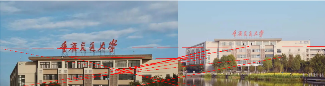
SIFT特征匹配结果:
4、实验总结
从实验结果明显可以看出,Harris的匹配点对数远远多于SIFT匹配点对数,但是精确度却不是很高,出现较多匹配错误的情况,但是可以发现在SIFT的特征匹配中,匹配的关键点很少,但是准确率非常高,关键点少的原因之音可能是最后的阈值设置过高,符合条件的关键点比较少。可以看到,拍的两张图片分别是左右半边,图书馆是对称结构,Harris出现匹配错位的情况非常多,但是在SIFT匹配中几乎没有出现错误的情况。可以看出,在多角点的复杂建筑图像中,SIFT的匹配性能要高于Harris。


暂无评论内容